LIF voltage traces and a recurrent network raster

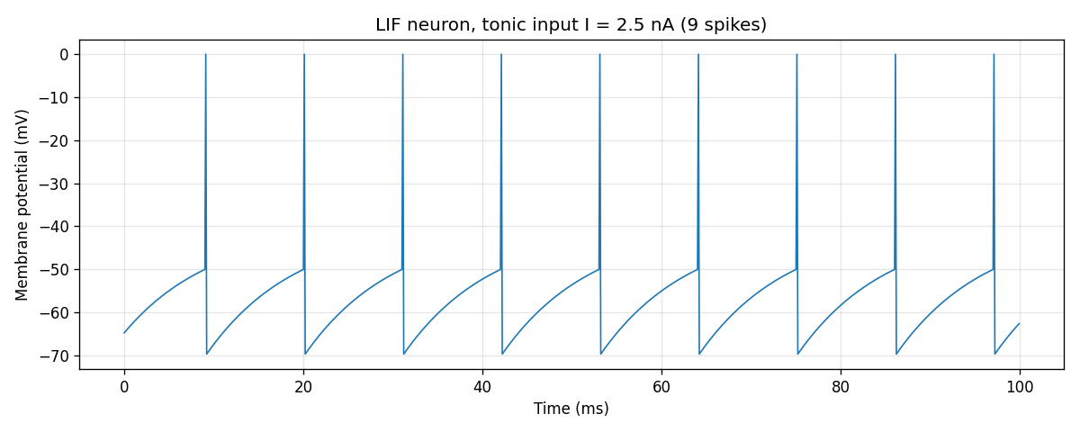
The leaky integrate-and-fire (LIF) model is the simplest spiking neuron worth taking seriously. Its membrane voltage decays toward a resting potential and is pushed around by injected current; when the voltage crosses a threshold the neuron emits a spike and resets.

The subthreshold dynamics are

with a spike-and-reset rule

The code integrates this with forward Euler at $\Delta t = 0.1\,\text{ms}$,

using $\tau_m = 10\,\text{ms}$, $V_\text{rest} = -65\,\text{mV}$, $V_\text{reset} = -70\,\text{mV}$, $V_\text{th} = -50\,\text{mV}$, $R_m = 10\,\text{M}\Omega$, and tonic input $I = 2.5\,\text{nA}$.

With a steady tonic input current above threshold, the neuron fires periodically. Each upward sweep is the membrane charging through its RC time constant; each vertical line is a reset after a spike.

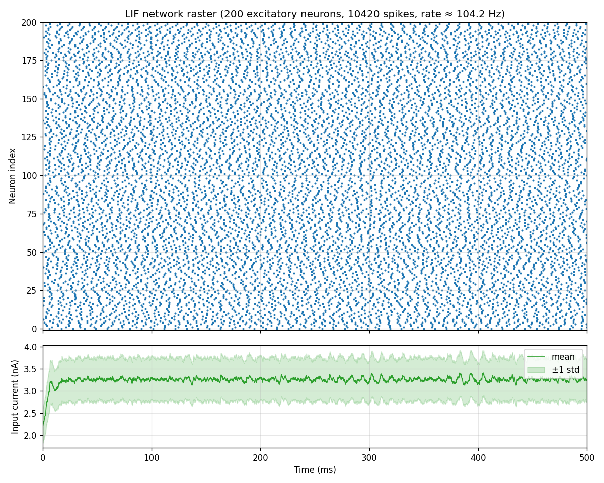
Connect 200 such neurons together with sparse, all-excitatory recurrence and noisy per-neuron bias currents, and the dynamics get more interesting. Each neuron $i$ obeys the same LIF dynamics, but with a total input current

with $\mu = 2.2\,\text{nA}$ and $\sigma = 0.4\,\text{nA}$. The synaptic current $s_i$ decays exponentially between spikes and is kicked by incoming spikes,

where $\tau_\text{syn} = 5\,\text{ms}$ and the weight matrix is $W_{ij} = w\, C_{ij}$ with $C_{ij} \sim \text{Bernoulli}(p_\text{conn})$, $w = 0.1$, $p_\text{conn} = 0.1$, and no self-connections. After each spike the neuron is held at $V_\text{reset}$ for a refractory period of $2\,\text{ms}$.

The raster below shows every spike from every neuron over half a second of simulated time; the panel underneath tracks the network’s mean total input current (bias plus decaying synaptic input), with the shaded band showing one standard deviation across the population.

Both figures were generated by running neuron lif and neuron net and copying the PNGs into this post’s asset directory.

LIF run parameters

Network run parameters